library(deSolve)
library(tidyverse)SD Tutorial 6: S-Shaped Growth — SIS Epidemic Model
Two interacting stocks, opposing flows, and the dynamics of infection
Required R packages
S-Shaped Growth Is a Behaviour, Not a Structure
In Tutorial 5 we saw S-shaped growth emerge from a single stock with a density-dependent deaths multiplier. This tutorial shows that the same characteristic behaviour can arise from a completely different mechanism — two interacting stocks with no lookup tables at all.
The key insight: S-shaped growth is a behaviour pattern, not a structure. Multiple mechanistically distinct systems can produce it.
The SIS Epidemic Structure
This model describes the spread of an illness through a fixed population of 100 people. There is no permanent immunity: once a sick person recovers, they return to the healthy pool and can be re-infected. This is known as an SIS (Susceptible → Infected → Susceptible) structure.
The two stocks are:
- Healthy People — those susceptible to infection
- Sick People — those currently infected
Two flows connect them in opposing directions:
- Catching Illness — moves people from Healthy to Sick; driven by contact between healthy and sick people
- Recovering — moves people from Sick back to Healthy; driven by the duration of illness
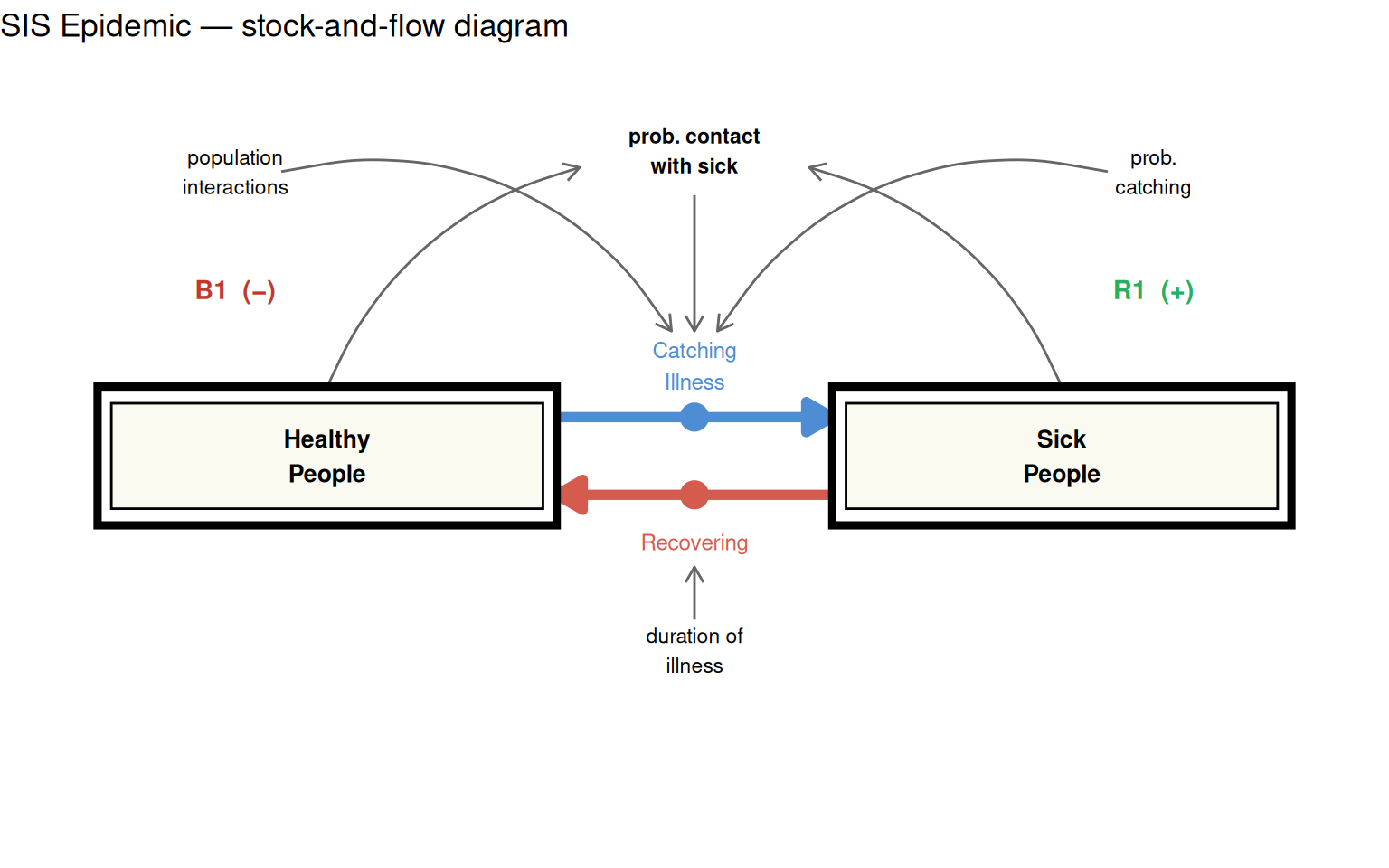
Two feedback loops drive this system:
- R1 (+): More sick people → more probability of contact with sick people → more probability of catching illness → more sick people. This reinforcing loop accelerates the epidemic.
- B1 (-): More healthy people → lower probability of contact with sick people → less catching illness → fewer sick people → fewer people recovering → fewer healthy people. This balancing loop controls disease spread over time.
Model Equations
The catching illness rate depends on three factors: the number of healthy people available to be infected, the probability of contact with a sick person (sick/total population), and the rate and likelihood of transmission on contact.
\[\text{Catching Illness} = \text{Healthy} \times \frac{\text{Sick}}{\text{Total Population}} \times \text{Population Interactions} \times P(\text{catching})\]
\[\text{Recovering} = \frac{\text{Sick}}{\text{Duration of Illness}}\]
The differential equations governing the two stocks are:
\[\frac{d(\text{Healthy})}{dt} = \text{Recovering} - \text{Catching Illness}\]
\[\frac{d(\text{Sick})}{dt} = \text{Catching Illness} - \text{Recovering}\]
Note that total population = Healthy + Sick is conserved — the model has no births or deaths, only movement between compartments.
Parameters
| Parameter | Symbol | Value | Units |
|---|---|---|---|
| Duration of illness | \(D\) | 0.5 | months |
| Population interactions | \(PI\) | 10 | contacts / person / month |
| Probability of catching | \(PC\) | 0.5 | dimensionless |
R Modelling Tutorial
Model function
The model follows the standard deSolve function signature. Variable names use the project’s prefix convention (s_ stocks, p_ parameters, c_ converters, f_ flows).
model <- function(time, stocks, params) {
  with(as.list(c(stocks, params)), {

    c_prob_contact_sick <- s_sick / (s_healthy + s_sick)

    f_catching_illness <- s_healthy * c_prob_contact_sick *
                          p_population_interactions * p_prob_catching   # people/month
    f_recovering    <- s_sick / p_duration_of_illness                # people/month

    ds_healthy_dt <- f_recovering - f_catching_illness
    ds_sick_dt    <- f_catching_illness - f_recovering

    return(list(c(ds_healthy_dt, ds_sick_dt),
                catching_illness = f_catching_illness,
                recovery_rate    = f_recovering))
  })
}
Parameters and simulation time
params <- c(p_duration_of_illness     = 0.5,   # months
            p_population_interactions = 10,    # contacts/person/month
            p_prob_catching           = 0.5)   # dimensionless

simtime <- seq(0, 5, by = 0.125)               # months
Single test run
Before running multiple scenarios, let us verify the model produces sensible output for one set of initial conditions: 10 sick people and 90 healthy people.
stocks_a <- c(s_healthy = 90, s_sick = 10)

test_run <- ode(y = stocks_a, times = simtime, func = model,
                parms = params, method = "rk4") %>%
  as_tibble() %>%
  pivot_longer(-time) %>%
  mutate(value = as.numeric(value),
         time  = as.numeric(time))

test_run %>%
  filter(name %in% c("s_healthy", "s_sick")) %>%
  ggplot(aes(x = time, y = value, colour = name)) +
  geom_line(linewidth = 0.9) +
  scale_colour_manual(values = c(s_healthy = "#4e8cd4", s_sick = "#d45b4e"),
                      labels = c(s_healthy = "Healthy People",
                                 s_sick    = "Sick People")) +
  labs(title  = "SIS epidemic — single run (10 sick, 90 healthy)",
       x      = "Months",
       y      = "People",
       colour = NULL)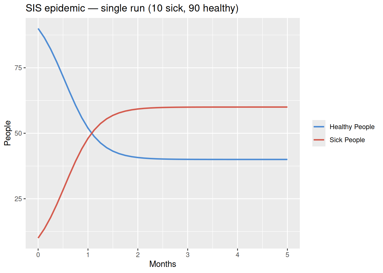
The system reaches a stable equilibrium rather than infecting the entire population. The epidemic overshoots slightly then settles — a classic S-shaped trajectory for sick people.
Exercise 2: four initial conditions
To understand how initial conditions affect behaviour, we run four scenarios matching Exercise 2 from the Road Maps source material. We wrap the simulation in a function and use purrr::pmap_dfr() to iterate across all four scenarios at once.
run_sis <- function(sim_id, init_healthy, init_sick,
                    start = 0, finish = 5, step = 0.125) {
  stocks <- c(s_healthy = init_healthy, s_sick = init_sick)
  sim_time <- seq(start, finish, by = step)

  ode(y = stocks, times = sim_time, func = model,
      parms = params, method = "rk4") %>%
    as_tibble() %>%
    pivot_longer(-time) %>%
    mutate(value = as.numeric(value),
           time  = as.numeric(time),
           run   = sim_id)
}
sim_results <- pmap_dfr(
list(
sim_id = c("a: 5 sick, 95 healthy",
"b: 0 sick — no epidemic",
"c: 55 sick, 45 healthy",
"d: 50 sick, 50 healthy"),
init_healthy = c(95, 100, 45, 50),
init_sick = c(5, 0, 55, 50)
),
.f = run_sis
)
glimpse(sim_results)Rows: 656
Columns: 4
$ time <dbl> 0.000, 0.000, 0.000, 0.000, 0.125, 0.125, 0.125, 0.125, 0.250, 0…
$ name <chr> "s_healthy", "s_sick", "catching_illness", "recovery_rate", "s_h…
$ value <dbl> 95.000000, 5.000000, 23.750000, 10.000000, 92.990980, 7.009020, …
$ run <chr> "a: 5 sick, 95 healthy", "a: 5 sick, 95 healthy", "a: 5 sick, 95…sim_results %>%
filter(name %in% c("s_healthy", "s_sick")) %>%
mutate(name = recode(name,
s_healthy = "Healthy People",
s_sick = "Sick People")) %>%
ggplot(aes(x = time, y = value, colour = run)) +
geom_line(linewidth = 0.8) +
facet_wrap(~name) +
labs(title = "Exercise 2 — four initial conditions",
x = "Months",
y = "People",
colour = "Run")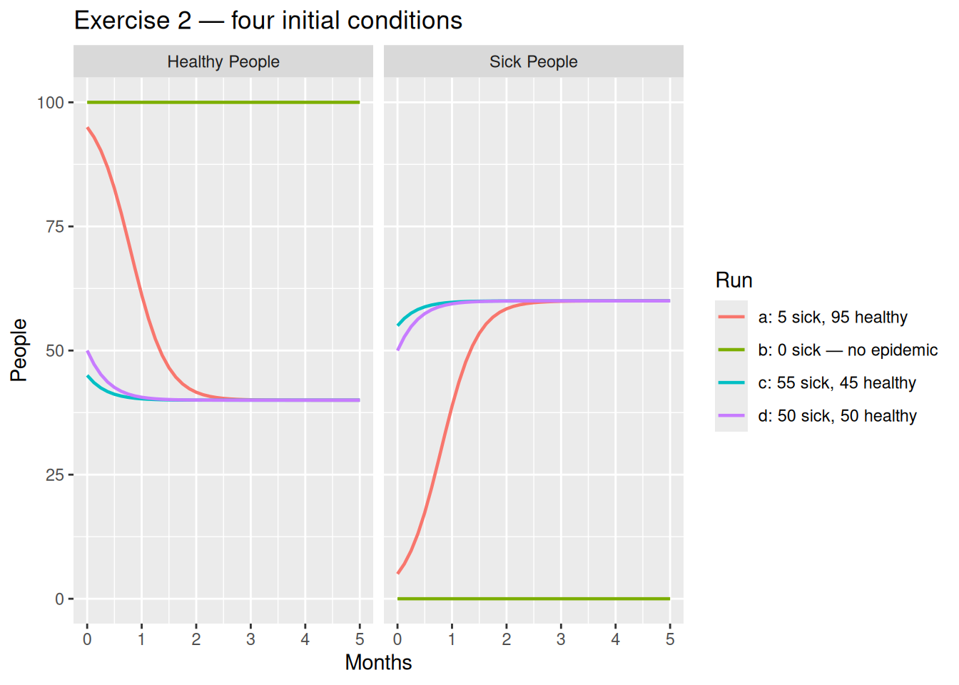
The four runs reveal the key behaviours of this system:
- Run a (5 sick) and run d (50 sick): both converge to the same equilibrium of 40 healthy / 60 sick, regardless of where they started. The system has a single stable attractor.
- Run c (55 sick): starts above the equilibrium sick count and decays back down to it — the epidemic recedes.
- Run b (0 sick): with no sick people to start, the positive feedback loop cannot ignite. Total population stays healthy — this is an unstable equilibrium at
Sick = 0.
Run e: terminal illness
What happens if there is no recovery? A terminal illness removes the balancing loop B1 entirely. Without recovery pulling people back to the healthy pool, the epidemic follows a pure S-curve until the entire population is sick.
model_no_recovery <- function(time, stocks, params) {
  with(as.list(c(stocks, params)), {

    c_total_population  <- s_healthy + s_sick
    c_prob_contact_sick <- s_sick / c_total_population

    f_catching_illness <- s_healthy * c_prob_contact_sick *
                          p_population_interactions * p_prob_catching
    f_recovering    <- 0

    ds_healthy_dt <- -f_catching_illness
    ds_sick_dt    <-  f_catching_illness

    return(list(c(ds_healthy_dt, ds_sick_dt),
                catching_illness = f_catching_illness,
                recovery_rate    = f_recovering))
  })
}
simtime_e <- seq(0, 8, by = 0.125) # extended to show full S-curve
run_e <- ode(y = c(s_healthy = 90, s_sick = 10), times = simtime_e,
func = model_no_recovery, parms = params, method = "rk4") %>%
as_tibble() %>%
pivot_longer(-time) %>%
mutate(value = as.numeric(value),
time = as.numeric(time))
run_e %>%
filter(name %in% c("s_healthy", "s_sick")) %>%
mutate(name = recode(name,
s_healthy = "Healthy People",
s_sick = "Sick People")) %>%
ggplot(aes(x = time, y = value, colour = name)) +
geom_line(linewidth = 0.9) +
scale_colour_manual(values = c("Healthy People" = "#4e8cd4",
"Sick People" = "#d45b4e")) +
labs(title = "Run e — terminal illness (no recovery)",
x = "Months",
y = "People",
colour = NULL)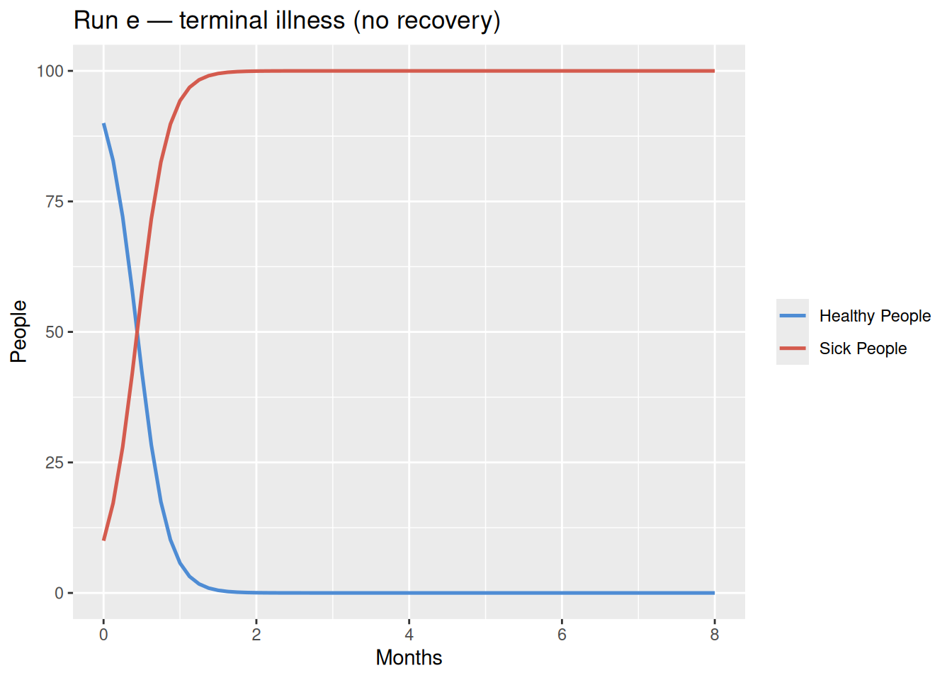
Without recovery, sick people grow in a classic S-shape — slow at first (few sick), then rapid (positive loop dominates), then levelling off as the healthy pool is exhausted (negative loop B2 dominates). The system reaches a new equilibrium of Sick = 100, Healthy = 0.
Conclusion
This tutorial demonstrated S-shaped growth emerging from a two-stock SIS epidemic structure. Several insights stand out:
S-shaped growth is a behaviour, not a structure. The same S-curve seen in the single-stock density model (Tutorial 5) arises here from a fundamentally different mechanism — the interaction between two populations.
The product of two stocks creates nonlinearity. The catching illness rate is proportional to
Healthy × (Sick/Total), which is what generates the characteristic S-shape without any lookup table.Initial conditions determine trajectory, not destination. All positive-\(S_0\) runs converge to the same equilibrium; only the path differs.
Removing recovery eliminates the stable interior equilibrium. Without recovery (run e), the only equilibrium is full infection — confirming that B1 is essential for containing the epidemic.