SD Tutorial 2: Behavior of First-Order Positive Feedback Systems

Sensitivity analysis using deSolve and purrr

Required R packages

library(deSolve)
library(tidyverse)

Generic structure system behavior

The generic structure of a first order positive system can be shown as follows.

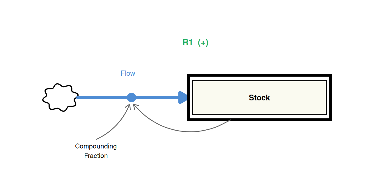
To explore the different behaviors possible from this system, we will use the R model developed in Tutorial 1. We’ll make some adjustments to the model, however, so we can easily run several simulations at once with different input values.

We will first experiment by testing the effects of changing the initial value of the stock. We’ll give the stock initial values of -200, -100, 0, 100, and 200 for simulation runs 1 through 5 respectively. The compounding fraction will be kept constant at 0.1.

R Modelling Tutorial

First, wrap up the entire simulation model into a single nested function. Variable names use the project’s prefix convention (s_ stocks, p_ parameters, c_ converters, f_ flows).

# define single function with all model parameters as arguments
first_order_pos_feedback <- function(sim = 1,
                                     stock,
                                     compounding_fraction,
                                     start,
                                     finish,
                                     step) {

  # model inputs
  sim_time <- seq(from = start,
                  to = finish,
                  by = step)
  stocks <- c(stock = stock)
  params <- c(compounding_fraction = compounding_fraction)  # (unit/unit)/time

  # define system model
  system_model <- function(time, stocks, params, sim){

    with(as.list(c(stocks, params)),

         {f_growing <- compounding_fraction * stock         # people/year
         ds_dt <- f_growing
         return(list(c(ds_dt),
                     change_in_stock = f_growing,
                     sim = sim))}
         )
  }

  # runs ode solver and tidy data
  sim_data <- ode(times = sim_time, y = stocks, parms = params,
                  func = system_model, method = "euler", sim = sim) %>%
    as_tibble() %>%
    relocate(sim, .before = time) %>%
    pivot_longer(-c(sim:time)) %>%
    mutate(value = as.numeric(value),
           time = as.numeric(time),
           sim = as.character(sim))

  return(sim_data)
}

Let us test our new function and plot one set of results to see how it works. Plot only the behavior of the stock.

# test simulation run 1
first_order_pos_feedback(stock = 200,
                         compounding_fraction = 0.1,
                         start = 0,
                         finish = 25,
                         step = 0.25) %>%
  filter(name == "stock") %>%
  ggplot(aes(x = time, y = value)) +
  geom_line(color = "grey25") +
  labs(title = "First-order positive feedback results",
       y = "stock value")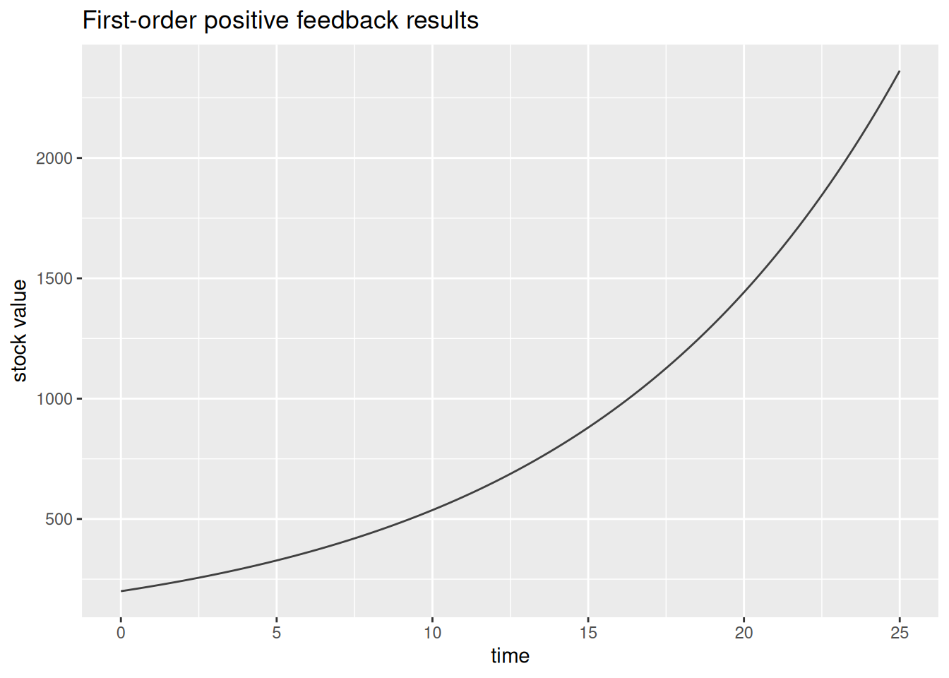

Now what we’d like to do is directly compare the results of running the simulation for the five initial values of the stock as mention above. We’ll accomplish this using the purrr package and iterating the function we just created over a list of initial values that we create.

# stock initial values
stocks_list <- c(-200, -100, 0, 100, 200)

# sim runs
sim_runs <- seq_along(stocks_list)

# map
sim_results <- pmap_dfr(list(sim = sim_runs,
                             stock = stocks_list),
                        .f = first_order_pos_feedback,
                        compounding_fraction = 0.1,
                        start = 0,
                        finish = 25,
                        step = 0.25)
# check results
glimpse(sim_results)

Rows: 1,010
Columns: 4
$ sim   <chr> "1", "1", "1", "1", "1", "1", "1", "1", "1", "1", "1", "1", "1",…
$ time  <dbl> 0.00, 0.00, 0.25, 0.25, 0.50, 0.50, 0.75, 0.75, 1.00, 1.00, 1.25…
$ name  <chr> "stock", "change_in_stock", "stock", "change_in_stock", "stock",…
$ value <dbl> -200.00000, -20.00000, -205.00000, -20.50000, -210.12500, -21.01…

Immediately notice the number of rows in this new data set. Using pmap_dfr we have concatenated by rows each subsequent simulation run. Let’s now plot all the results so we can compare the effects of the different stock initial values on the system behavior.

sim_results %>%
  filter(name == "stock") %>%
  ggplot(aes(y = value, x = time, color = sim)) +
  geom_line() +
  labs(title = "Stock initial value sensitivity test",
       y = "stock value")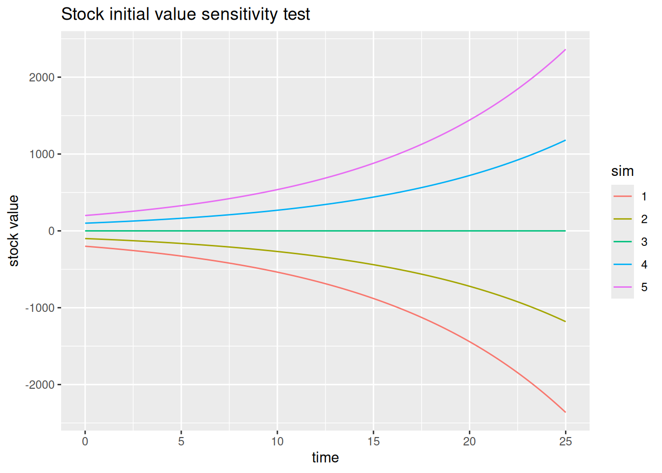

Let us now explore what accelerates or slows the exponential growth of a system. We will study the effect of changing the value of the compounding fraction while keeping the initial value of the stock constant. The compounding fraction will take values of 0, 0.1, 0.2, 0.3, and 0.4 for runs 1 through 5 respectively. The initial value of the stock will be kept constant at 100.

# compounding fraction values
fraction_list <- c(0, 0.1, 0.2, 0.3, 0.4)

# sim runs
sim_runs <- seq_along(fraction_list)

# map and plot
pmap_dfr(list(sim = sim_runs,
              compounding_fraction = fraction_list),
         .f = first_order_pos_feedback,
         stock = 100,
         start = 0,
         finish = 25,
         step = 0.25) %>%
  filter(name == "stock") %>%
  ggplot(aes(y = value, x = time, color = sim)) +
  geom_line() +
  scale_y_continuous(limits = c(0, 5000)) +
  labs(title = "Compounding fraction sensitivity test",
       y = "stock value")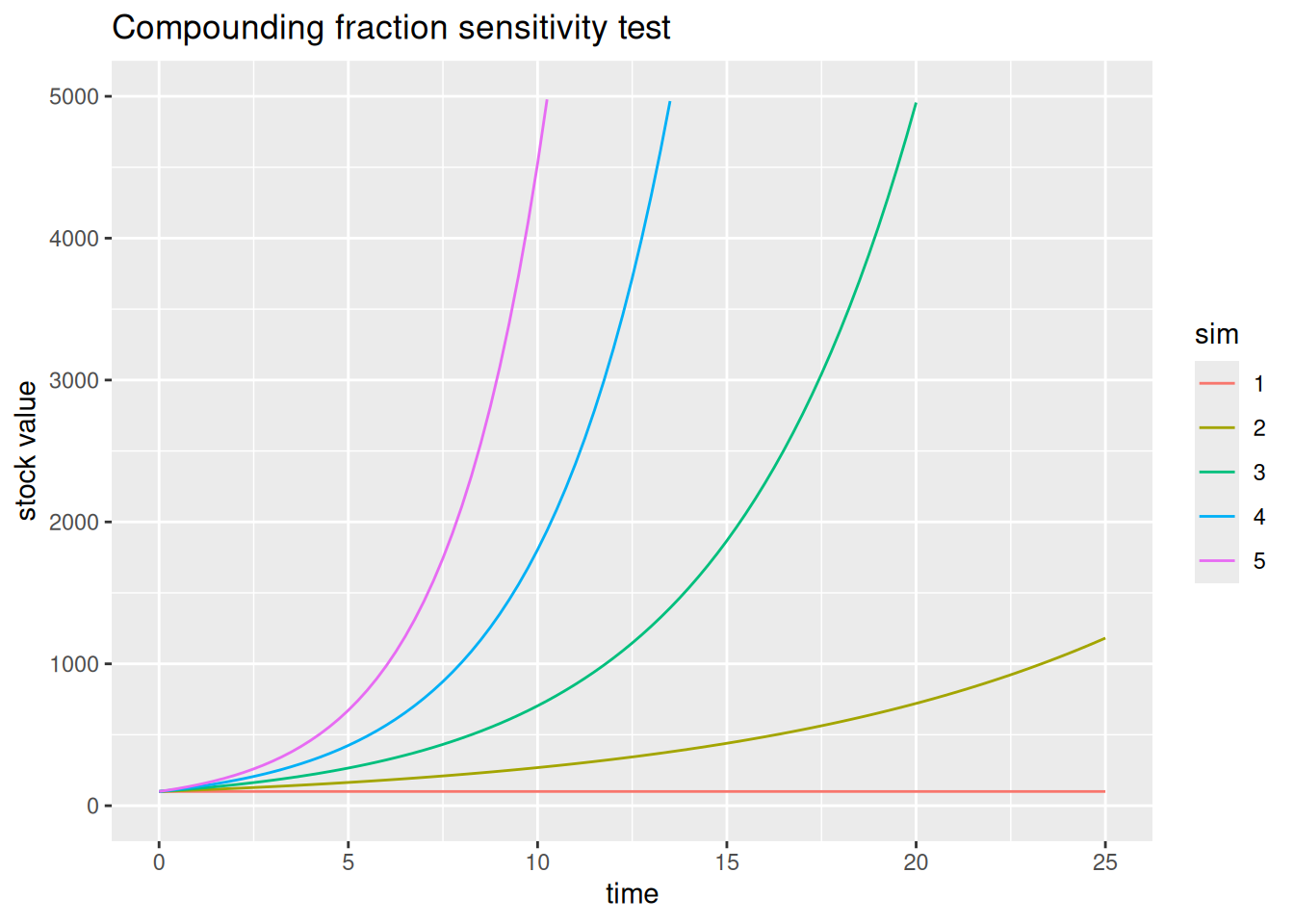

Conclusion

Understanding how to code and perform sensitivity tests is extremely important in SD modelling. Once you introduce feedback into a system, behavior can change dramatically with only slight tweaks of parameters. Sensitivity testing can help you understand the key leverage points in your system.